Bayesian Multiple Regression Example

import arviz as az
import bambi as bmb
import numpy as np
import pandas as pd
import pymc3 as pm
import seaborn as sns
import statsmodels.api as sm

az.style.use('arviz-darkgrid')

Load and examine Eugene-Springfield community sample data

data = pd.read_csv('data/ESCS.csv')
np.round(data.describe(), 2)

	drugs	n	e	o	a	c	hones	emoti	extra	agree	consc	openn
count	604.00	604.00	604.00	604.00	604.00	604.00	604.00	604.00	604.00	604.00	604.00	604.00
mean	2.21	80.04	106.52	113.87	124.63	124.23	3.89	3.18	3.21	3.13	3.57	3.41
std	0.65	23.21	19.88	21.12	16.67	18.69	0.45	0.46	0.53	0.47	0.44	0.52
min	1.00	23.00	42.00	51.00	63.00	44.00	2.56	1.47	1.62	1.59	2.00	1.28
25%	1.71	65.75	93.00	101.00	115.00	113.00	3.59	2.88	2.84	2.84	3.31	3.06
50%	2.14	76.00	107.00	112.00	126.00	125.00	3.88	3.19	3.22	3.16	3.56	3.44
75%	2.64	93.00	120.00	129.00	136.00	136.00	4.20	3.47	3.56	3.44	3.84	3.75
max	4.29	163.00	158.00	174.00	171.00	180.00	4.94	4.62	4.75	4.44	4.75	4.72

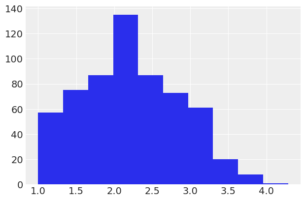
It’s always a good idea to start off with some basic plotting. Here’s what our outcome variable ‘drugs’ (some index of self-reported illegal drug use) looks like:

data['drugs'].hist();

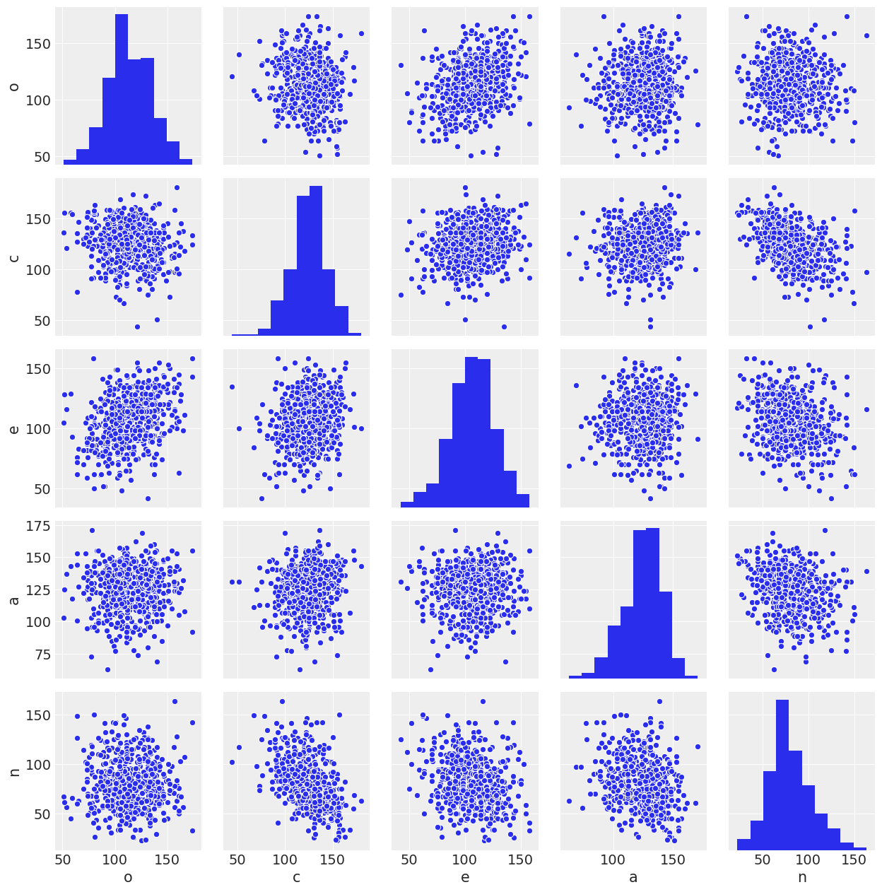
The five predictor variables that we’ll use are sum-scores measuring participants’ standings on the Big Five personality dimensions. The dimensions are: - O = Openness to experience - C = Conscientiousness - E = Extraversion - A = Agreeableness - N = Neuroticism

Here’s what our predictors look like:

sns.pairplot(data[['o','c','e','a','n']]);

Specify model and examine priors

We’re going to fit a pretty straightforward multiple regression model predicting drug use from all 5 personality dimension scores. It’s simple to specify the model using a familiar formula interface. Here we tell bambi to run two parallel Markov Chain Monte Carlo (MCMC) chains, each one drawing 2000 samples from the joint posterior distribution of all the parameters.

model = bmb.Model(data)
fitted = model.fit('drugs ~ o + c + e + a + n', samples=1000, tune=1000, init='adapt_diag')

INFO:numexpr.utils:NumExpr defaulting to 4 threads.
Auto-assigning NUTS sampler...
INFO:pymc3:Auto-assigning NUTS sampler...
Initializing NUTS using adapt_diag...
INFO:pymc3:Initializing NUTS using adapt_diag...
Multiprocess sampling (2 chains in 2 jobs)
INFO:pymc3:Multiprocess sampling (2 chains in 2 jobs)
NUTS: [drugs_sd, n, a, e, c, o, Intercept]
INFO:pymc3:NUTS: [drugs_sd, n, a, e, c, o, Intercept]

100.00% [4000/4000 00:21<00:00 Sampling 2 chains, 1 divergences]

Great! But this is a Bayesian model, right? What about the priors?

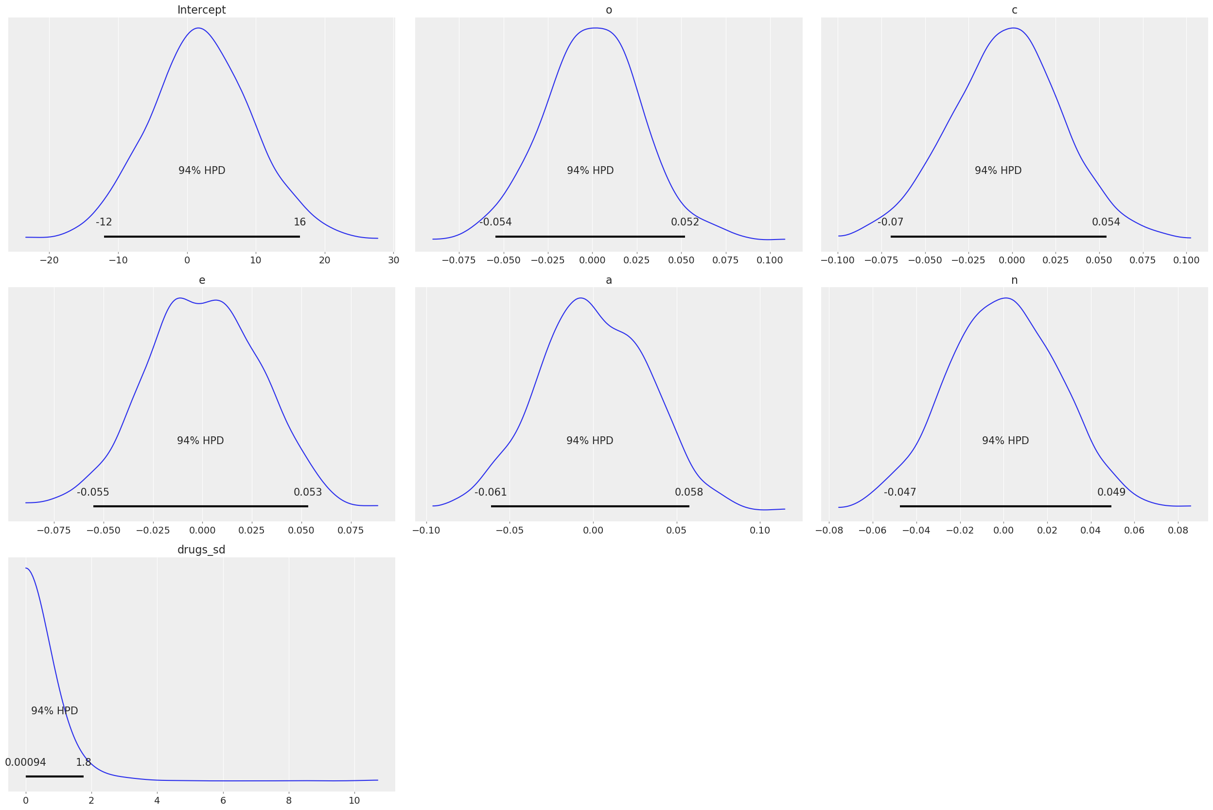
If no priors are given explicitly by the user, then bambi chooses smart default priors for all parameters of the model based on the implied partial correlations between the outcome and the predictors. Here’s what the default priors look like in this case – the plots below show 1000 draws from each prior distribution:

model.plot();

# Normal priors on the coefficients
{x.name:x.prior.args for x in model.terms.values()}

{'Intercept': {'mu': array([2.21014664]), 'sd': array([7.49872452])},
 'o': {'mu': array([0]), 'sd': array([0.02706881])},
 'c': {'mu': array([0]), 'sd': array([0.03237049])},
 'e': {'mu': array([0]), 'sd': array([0.02957414])},
 'a': {'mu': array([0]), 'sd': array([0.03183623])},
 'n': {'mu': array([0]), 'sd': array([0.02641989])}}

# Uniform prior on the residual standard deviation
model.y.prior.args['sd'].args

{'nu': array(4), 'sd': array(0.64877877)}

Some more info about the default prior distributions can be found in this technical paper.

Notice the small SDs of the slope priors. This is due to the relative scales of the outcome and the predictors: remember from the plots above that the outcome, drugs, ranges from 1 to about 4, while the predictors all range from about 20 to 180 or so. So a one-unit change in any of the predictors – which is a trivial increase on the scale of the predictors – is likely to lead to a very small absolute change in the outcome. Believe it or not, these priors are actually quite wide on the partial correlation scale!

Examine the model results

Let’s start with a pretty picture of the parameter estimates!

az.plot_trace(fitted);

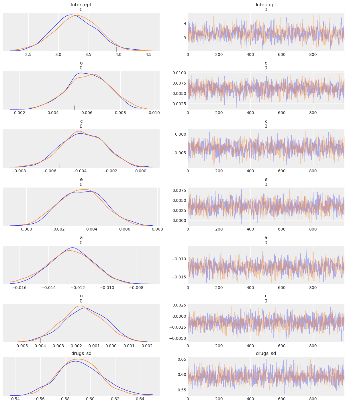
The left panels show the marginal posterior distributions for all of the model’s parameters, which summarize the most plausible values of the regression coefficients, given the data we have now observed. These posterior density plots show two overlaid distributions because we ran two MCMC chains. The panels on the right are “trace plots” showing the sampling paths of the two MCMC chains as they wander through the parameter space.

A much more succinct (non-graphical) summary of the parameter estimates can be found like so:

az.summary(fitted)

	mean	sd	hpd_3%	hpd_97%	mcse_mean	mcse_sd	ess_mean	ess_sd	ess_bulk	ess_tail	r_hat
Intercept[0]	3.291	0.364	2.630	3.991	0.013	0.009	797.0	791.0	799.0	839.0	1.0
o[0]	0.006	0.001	0.004	0.008	0.000	0.000	1228.0	1228.0	1225.0	1476.0	1.0
c[0]	-0.004	0.001	-0.006	-0.001	0.000	0.000	962.0	886.0	962.0	856.0	1.0
e[0]	0.003	0.001	0.001	0.006	0.000	0.000	1615.0	1490.0	1620.0	1485.0	1.0
a[0]	-0.012	0.002	-0.015	-0.010	0.000	0.000	1009.0	991.0	1013.0	980.0	1.0
n[0]	-0.001	0.001	-0.004	0.001	0.000	0.000	1256.0	1190.0	1255.0	1129.0	1.0
drugs_sd	0.592	0.017	0.560	0.624	0.000	0.000	1562.0	1562.0	1548.0	1290.0	1.0

When there are multiple MCMC chains, the default summary output includes some basic convergence diagnostic info (the effective MCMC sample sizes and the Gelman-Rubin “R-hat” statistics), although in this case it’s pretty clear from the trace plots above that the chains have converged just fine.

Summarize effects on partial correlation scale

samples = fitted.posterior

It turns out that we can convert each regresson coefficient into a partial correlation by multiplying it by a constant that depends on (1) the SD of the predictor, (2) the SD of the outcome, and (3) the degree of multicollinearity with the set of other predictors. Two of these statistics are actually already computed and stores in the fitted model object, in a dictionary called dm_statistics (for design matrix statistics), because they are used internally. The others we will compute manually.

# the names of the predictors
varnames = ['o', 'c', 'e', 'a', 'n']

# compute the needed statistics
r2_x = model.dm_statistics['r2_x']
sd_x = model.dm_statistics['sd_x']
r2_y = pd.Series([sm.OLS(endog=data['drugs'],
                         exog=sm.add_constant(data[[p for p in varnames if p != x]])).fit().rsquared
                  for x in varnames], index=varnames)
sd_y = data['drugs'].std()

# compute the products to multiply each slope with to produce the partial correlations
slope_constant = sd_x[varnames] * (1 - r2_x[varnames])**.5 \
    / sd_y / (1 - r2_y)**.5
slope_constant

o    32.392557
c    27.674284
e    30.305117
a    26.113299
n    34.130431
dtype: float64

Now we just multiply each sampled regression coefficient by its corresponding slope_constant to transform it into a sampled partial correlation coefficient.

pcorr_samples = samples[varnames] * slope_constant

And voilà! We now have a joint posterior distribution for the partial correlation coefficients. Let’s plot the marginal posterior distributions:

for idx, (k, v) in enumerate(pcorr_samples.items()):
    ax = az.plot_kde(v, label=k, plot_kwargs={'color':f'C{idx}'})
ax.axvline(x=0, color='k', linestyle='--');

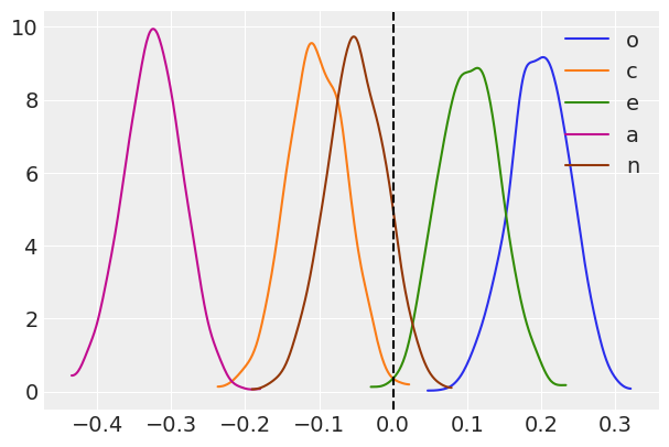
The means of these distributions serve as good point estimates of the partial correlations:

pcorr_samples.mean(dim=['chain', 'draw']).squeeze(drop=True)

<xarray.Dataset>
Dimensions:  ()
Data variables:
    o        float64 0.197
    c        float64 -0.104
    e        float64 0.1029
    a        float64 -0.3245
    n        float64 -0.0509

Naturally, these results are consistent with the OLS results. For example, we can see that these estimated partial correlations are roughly proportional to the t-statistics from the corresponding OLS regression:

sm.OLS(endog=data['drugs'], exog=sm.add_constant(
    data[varnames])).fit().summary()

OLS Regression Results

Dep. Variable:	drugs	R-squared:	0.176
Model:	OLS	Adj. R-squared:	0.169
Method:	Least Squares	F-statistic:	25.54
Date:	Fri, 21 Feb 2020	Prob (F-statistic):	2.16e-23
Time:	20:17:38	Log-Likelihood:	-536.75
No. Observations:	604	AIC:	1086.
Df Residuals:	598	BIC:	1112.
Df Model:	5
Covariance Type:	nonrobust

	coef	std err	t	P>|t|	[0.025	0.975]
const	3.3037	0.360	9.188	0.000	2.598	4.010
o	0.0061	0.001	4.891	0.000	0.004	0.008
c	-0.0038	0.001	-2.590	0.010	-0.007	-0.001
e	0.0034	0.001	2.519	0.012	0.001	0.006
a	-0.0124	0.001	-8.391	0.000	-0.015	-0.010
n	-0.0015	0.001	-1.266	0.206	-0.004	0.001

Omnibus:	10.273	Durbin-Watson:	1.959
Prob(Omnibus):	0.006	Jarque-Bera (JB):	7.926
Skew:	0.181	Prob(JB):	0.0190
Kurtosis:	2.572	Cond. No.	3.72e+03

Warnings:
[1] Standard Errors assume that the covariance matrix of the errors is correctly specified.
[2] The condition number is large, 3.72e+03. This might indicate that there are
strong multicollinearity or other numerical problems.

Relative importance: Which predictors have the strongest effects (defined in terms of partial \(\eta^2\))?

The partial \(\eta^2\) statistics for each predictor are just the squares of the partial correlation coefficients, so it’s easy to get posteriors on that scale too:

for idx, (k, v) in enumerate(pcorr_samples.items()):
    ax = az.plot_kde(v**2, label=k, plot_kwargs={'color':f'C{idx}'})
    ax.set_ylim(0, 80)

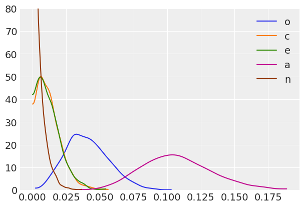
With these posteriors we can ask: What is the probability that the partial \(\eta^2\) for Openness (yellow) is greater than the partial \(\eta^2\) for Conscientiousness (green)?

For each predictor, what is the probability that it has the largest \(\eta^2\)?

pc_df = pcorr_samples.to_dataframe()
(pc_df**2).idxmax(axis=1).value_counts() / len(pc_df.index)

a    0.994
o    0.006
dtype: float64

Agreeableness is clearly the strongest predictor of drug use among the Big Five personality traits, but it’s still not a particularly strong predictor in an absolute sense. Walter Mischel famously claimed that it is rare to see correlations between personality measurse and relevant behavioral outcomes exceed 0.3. In this case, the probability that the agreeableness partial correlation exceeds 0.3 is:

(np.abs(pcorr_samples['a']) > .3).mean()

<xarray.DataArray 'a' ()>
array(0.7315)

Bayesian/Frequentist Tutorial Bayesian Workflow Example (Police Officer’s Dilemma)