Bayesian Logistic Regression Example

# Author: jake-westfall
# Created At: Sep 11, 2016
# Last Run: Mar 27, 2019

import bambi as bmb
import pandas as pd
import numpy as np
import matplotlib.pyplot as plt

Load and examine American National Election Studies (ANES) data

These data are from the 2016 pilot study. The full study consisted of 1200 people, but here we’ve selected the subset of 487 people who responded to a question about whether they would vote for Hillary Clinton or Donald Trump.

data = pd.read_csv('data/ANES_2016_pilot.csv')
data.head()

	vote	age	party_id
0	clinton	56	democrat
1	trump	65	republican
2	clinton	80	democrat
3	trump	38	republican
4	trump	60	republican

Our outcome variable is vote, which gives peoples’ responses to the following question prompt:

“If the 2016 presidential election were between Hillary Clinton for the Democrats and Donald Trump for the Republicans, would you vote for Hillary Clinton, Donald Trump, someone else, or probably not vote?”

data['vote'].value_counts()

clinton         215
trump           158
someone_else     48
Name: vote, dtype: int64

The two predictors we’ll examine are a respondent’s age and their political party affiliation, party_id, which is their response to the following question prompt:

“Generally speaking, do you usually think of yourself as a Republican, a Democrat, an independent, or what?”

data['party_id'].value_counts()

democrat       186
independent    138
republican      97
Name: party_id, dtype: int64

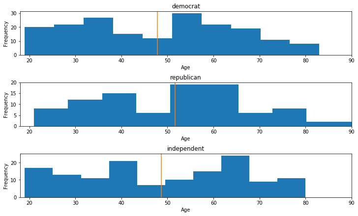
These two predictors are somewhat correlated, but not all that much:

fig, ax = plt.subplots(3, figsize=(10, 6), constrained_layout=True)
key = dict(zip(data['party_id'].unique(), range(3)))
for label, df in data.groupby('party_id'):
    ax[key[label]].hist(df['age'])
    ax[key[label]].set_xlim([18, 90])
    ax[key[label]].set_xlabel('Age')
    ax[key[label]].set_ylabel('Frequency')
    ax[key[label]].set_title(label)
    ax[key[label]].axvline(df['age'].mean(), color='C1')

We can get a pretty clear idea of how party identification is related to voting intentions by just looking at a contingency table for these two variables:

pd.crosstab(data['vote'], data['party_id'])

party_id	democrat	independent	republican
vote
clinton	159	51	5
someone_else	10	22	16
trump	17	65	76

But our main question here will be: How is respondent age related to voting intentions, and is this relationship different for different party affiliations? For this we will need logistic regression.

Build clinton_model

To keep this simple, let’s look at only the data from people who indicated that they would vote for either Clinton or Trump, and we’ll model the probability of voting for Clinton.

clinton_data = data.loc[data['vote'].isin(['clinton', 'trump']), :]
clinton_data.head()

	vote	age	party_id
0	clinton	56	democrat
1	trump	65	republican
2	clinton	80	democrat
3	trump	38	republican
4	trump	60	republican

Specifying and fitting the model is simple. Notice the (optional) syntax that we use on the left-hand-side of the formula: We say vote[clinton] to instruct bambi that we wish the model the probability that vote=='clinton', rather than the probability that vote=='trump'. If we leave this unspecified, bambi will just pick one of the events to model, but will inform you which one it picked when you build the model (and again when you look at model summaries.)

When fitting models using the pymc3 backend, the default estimation strategy is to start with an identity mass matrix, but add uniform jitter in [-1, 1] and then adapt a diagonal based on the variance of the tuning samples. This generally works quite well, but occasionally it can fails. That’s what was happening for this particular data set and model, so below we disable the jitter+adapt_diag initialization by changing from init='auto' (the default) to init=None, which tells the pymc3 backend to jump straight to the MCMC sampling.

clinton_model = bmb.Model(clinton_data)
clinton_fitted = clinton_model.fit('vote[clinton] ~ party_id + party_id:age',
                                   family='bernoulli', samples=1000, init=None)

/home/osvaldo/anaconda3/lib/python3.7/site-packages/pandas/core/frame.py:3140: SettingWithCopyWarning:
A value is trying to be set on a copy of a slice from a DataFrame.
Try using .loc[row_indexer,col_indexer] = value instead

See the caveats in the documentation: http://pandas.pydata.org/pandas-docs/stable/indexing.html#indexing-view-versus-copy
  self[k1] = value[k2]
/home/osvaldo/proyectos/00_PyMC3/bambi/bambi/models.py:228: UserWarning: Modeling the probability that vote=='clinton'
  self.y.name, str(self.clean_data[self.y.name].iloc[event])))
Sequential sampling (2 chains in 1 job)
INFO:pymc3:Sequential sampling (2 chains in 1 job)
NUTS: [party_id:age, party_id, Intercept]
INFO:pymc3:NUTS: [party_id:age, party_id, Intercept]
100%|██████████| 1500/1500 [00:09<00:00, 150.68it/s]
100%|██████████| 1500/1500 [00:07<00:00, 178.18it/s]

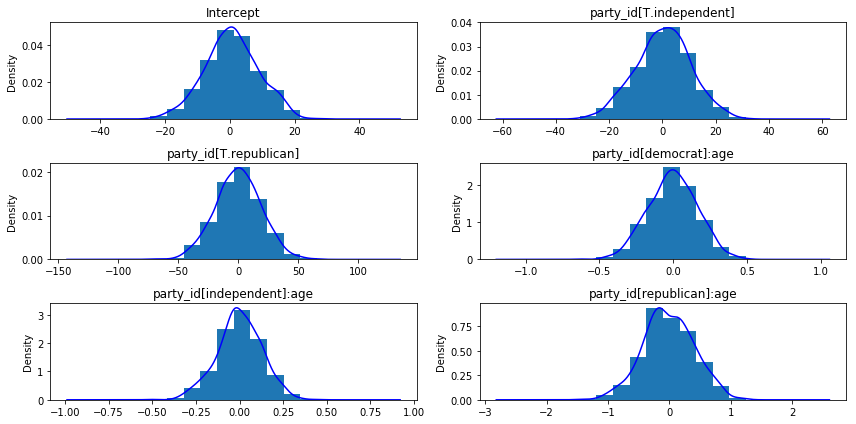
Since we didn’t explicitly set any of the prior distributions, here’s a view of what the default priors look like for all parameters:

clinton_model.plot();

{x.name: x.prior.args for x in clinton_model.terms.values()}

{'Intercept': {'mu': array([0.308043]), 'sd': array([8.39859892])},
 'party_id': {'mu': array([0, 0]), 'sd': array([10.51415445, 18.72417819])},
 'party_id:age': {'mu': array([0, 0, 0]),
  'sd': array([0.16748696, 0.12909332, 0.40771782])}}

Some more info about these default priors can be found in this technical paper.

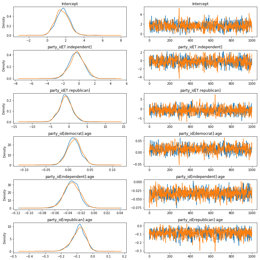
Now let’s check out the the results!

clinton_fitted.plot();

/home/osvaldo/proyectos/00_PyMC3/bambi/bambi/results.py:272: UserWarning: Modeling the probability that vote=='clinton'
  str(self.model.clean_data[self.model.y.name][event])))

clinton_fitted.summary()

/home/osvaldo/proyectos/00_PyMC3/bambi/bambi/results.py:362: UserWarning: Modeling the probability that vote=='clinton'
  str(self.model.clean_data[self.model.y.name][event])))

	mean	sd	hpd0.95_lower	hpd0.95_upper	effective_n	gelman_rubin
Intercept	1.673466	0.722605	0.277238	3.056835	751.509276	1.001686
party_id[T.independent]	-0.257464	0.905416	-2.092994	1.437578	778.058909	1.000464
party_id[T.republican]	-0.836706	1.704087	-4.237234	2.509791	957.738235	0.999702
party_id[democrat]:age	0.013165	0.015017	-0.018260	0.040125	781.775481	1.002113
party_id[independent]:age	-0.033724	0.011622	-0.057702	-0.012127	1040.377204	1.000000
party_id[republican]:age	-0.088576	0.042174	-0.178261	-0.016247	882.466245	0.999508

Run Inference

Grab the posteriors samples of the age slopes for the three party_id categories.

parties = ['democrat', 'independent', 'republican']
dem, ind, rep = [clinton_fitted.to_df()['party_id[{}]:age'.format(x)]
                 for x in parties]

for x in [dem, ind, rep]:
    x.plot(kind='kde', xlim=[-.2, .1])
plt.legend(loc='upper left')

<matplotlib.legend.Legend at 0x7f1160ff4ba8>

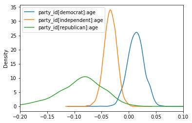
What is the probability that the Democrat slope is greater than the Republican slope?

(dem > rep).mean()

0.9965

Probability that the Democrat slope is greater than the Independent slope?

(dem > ind).mean()

0.9955

Probability that the Independent slope is greater than the Republican slope?

(ind > rep).mean()

0.904

Probability that the Democrat slope is greater than 0?

(dem > 0).mean()

0.8155

Probability that the Republican slope is less than 0?

(rep < 0).mean()

0.9925

Probability that the Independent slope is less than 0?

(ind < 0).mean()

0.9985

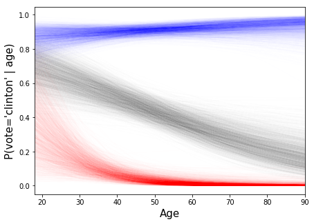
Spaghetti plot of model predictions

Grab all the MCMC samples.

trace_df = clinton_fitted.to_df()
trace_df.head()

	Intercept	party_id[T.independent]	party_id[T.republican]	party_id[democrat]:age	party_id[independent]:age	party_id[republican]:age
0	2.007555	0.789489	-1.173264	0.006203	-0.059276	-0.086375
1	2.295731	-0.638624	-1.309273	0.001157	-0.040808	-0.097659
2	2.396372	-0.631300	-0.980364	0.001990	-0.040614	-0.090759
3	2.027815	-1.264644	1.288043	0.008655	-0.025525	-0.159017
4	2.050935	-0.979028	1.119187	0.006341	-0.023220	-0.166833

Separate this into two DataFrames, one containing the intercept for each party_id, the other containing the age slopes for each party_id.

slopes = trace_df.iloc[:, -3:]
intercepts = pd.DataFrame({
    'dem': trace_df['Intercept'],
    'ind': trace_df['Intercept'] + trace_df['party_id[T.independent]'],
    'rep': trace_df['Intercept'] + trace_df['party_id[T.republican]']
})

Compute the predicted values for each posterior sample.

def invlogit(x): return 1/(1+np.exp(-x))


X = np.hstack([np.array([1]*len(np.arange(18, 91)))[:, None],
               np.arange(18, 91)[:, None]])
yhat = [invlogit(np.dot(X, np.vstack([intercepts.iloc[:, i], slopes.iloc[:, i]])))
        for i in range(3)]

Make the plot!

fig, axes = plt.subplots(figsize=(7, 5))

cols = ['b', 'g', 'r']
for i in range(3):
    for t in range(len(trace_df.index)):
        axes.plot(X[:, 1], yhat[i][:, t], alpha=.005, color=cols[i])
axes.set_ylabel('P(vote=\'clinton\' | age)', fontsize=15)
axes.set_xlabel('Age', fontsize=15)
axes.set_xlim(18, 90)

(18, 90)

Examples Bayesian/Frequentist Tutorial