Bayesian/Frequentist Tutorial
[ ]:
# Author: ejolly
# Created At: Jul 22, 2018
# Last Run: Jul 22, 2018
[24]:
import numpy as np
import pandas as pd
import matplotlib.pyplot as plt
import seaborn as sns
from pymer4.simulate import simulate_lm, simulate_lmm
import os
from glob import glob
%matplotlib inline
Generate t-test data
[86]:
a = np.random.normal(5,2,1000)
b = np.random.normal(8,2.5,1000)
df = pd.DataFrame({'Group':['a']*1000 + ['b']*1000,'Val':np.hstack([a,b])})
[87]:
df.groupby('Group').describe()
[87]:
| Val | ||||||||
|---|---|---|---|---|---|---|---|---|
| count | mean | std | min | 25% | 50% | 75% | max | |
| Group | ||||||||
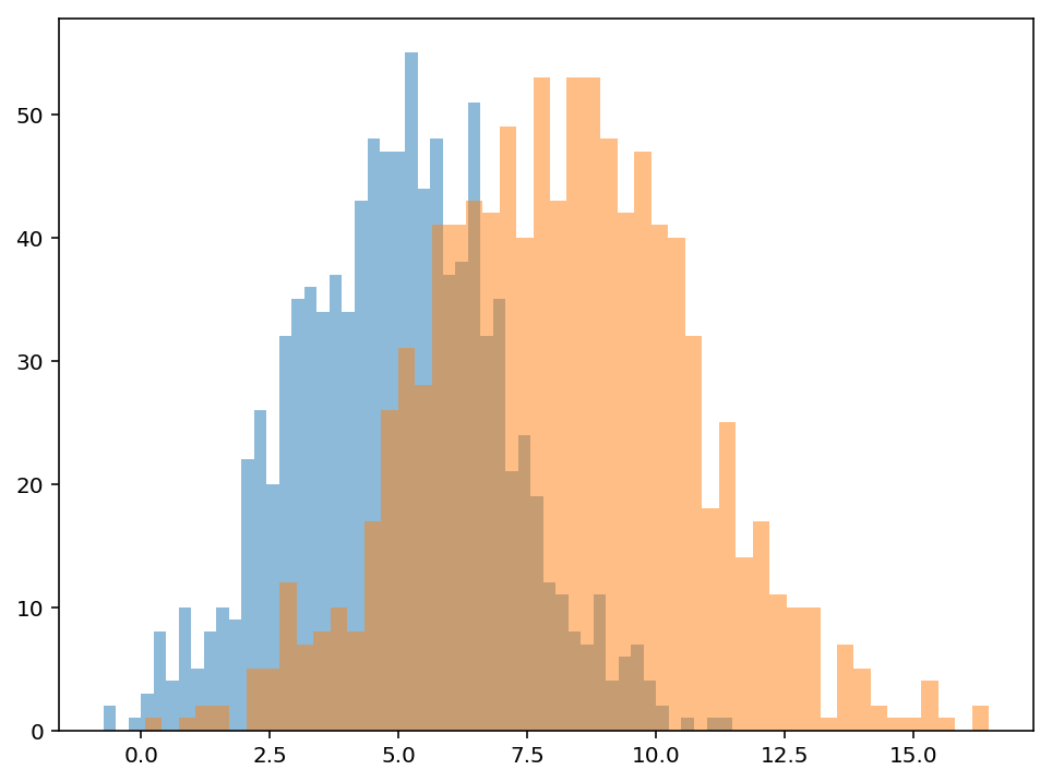
| a | 1000.0 | 4.980000 | 2.014565 | -0.732913 | 3.518155 | 5.013075 | 6.387810 | 11.466186 |
| b | 1000.0 | 8.129861 | 2.559710 | 0.074312 | 6.338794 | 8.150710 | 9.877882 | 16.458058 |
[88]:
f,ax = plt.subplots(1,1,figsize=(8,6))
ax.hist(a,alpha=.5,bins=50);
ax.hist(b,alpha=.5,bins=50);
Frequentist
Since this analysis is relateively straightforward we can perform a between groups t-test using scipy
[89]:
from scipy.stats import ttest_ind
ttest_ind(b,a)
[89]:
Ttest_indResult(statistic=30.57888496642679, pvalue=8.697871985710429e-169)
We can also set this up as a dummy-coded univariate regression model which is identical
[90]:
# Using the pymer4 package, but we could have used statsmodels instead
from pymer4.models import Lm
model = Lm('Val ~ Group',data=df)
model.fit()
Formula: Val ~ Group

Family: gaussian

Std-errors: non-robust  CIs: standard 95%       Inference: parametric

Number of observations: 2000     R^2: 0.319      R^2_adj: 0.318

Log-likelihood: -4505.582        AIC: 9015.163   BIC: 9026.365

Fixed effects:
[90]:
| Estimate | 2.5_ci | 97.5_ci | SE | DF | T-stat | P-val | Sig | |
|---|---|---|---|---|---|---|---|---|
| Intercept | 4.98 | 4.837 | 5.123 | 0.073 | 1998 | 68.371 | 0.0 | *** |
| Group[T.b] | 3.15 | 2.948 | 3.352 | 0.103 | 1998 | 30.579 | 0.0 | *** |
Bayesian
We can compute the equivalent dummy-coded regression model to estimate with bambi and the pymc3 backend
[91]:
from bambi import Model
import pymc3 as pm
import bambi

b_model = Model(df)
res_b = b_model.fit('Val ~ Group',samples=1000,chains=3)
Auto-assigning NUTS sampler...
Initializing NUTS using advi...
Average Loss = 4,542.7:  22%|██▏       | 11113/50000 [00:06<00:22, 1709.95it/s]
Convergence archived at 11300
Interrupted at 11,299 [22%]: Average Loss = 5,277
Multiprocess sampling (3 chains in 3 jobs)
NUTS: [Val_sd_interval__, Group, Intercept]
100%|██████████| 1500/1500 [00:01<00:00, 844.89it/s]
[93]:
# Here's the setup for the model
b_model.backend.model
[93]:
[94]:
# Model priors
b_model.plot();
/Users/Esh/anaconda3/lib/python3.6/site-packages/matplotlib/axes/_axes.py:6462: UserWarning: The 'normed' kwarg is deprecated, and has been replaced by the 'density' kwarg.
  warnings.warn("The 'normed' kwarg is deprecated, and has been "
/Users/Esh/anaconda3/lib/python3.6/site-packages/matplotlib/axes/_axes.py:6462: UserWarning: The 'normed' kwarg is deprecated, and has been replaced by the 'density' kwarg.
  warnings.warn("The 'normed' kwarg is deprecated, and has been "
/Users/Esh/anaconda3/lib/python3.6/site-packages/matplotlib/axes/_axes.py:6462: UserWarning: The 'normed' kwarg is deprecated, and has been replaced by the 'density' kwarg.
  warnings.warn("The 'normed' kwarg is deprecated, and has been "

[95]:
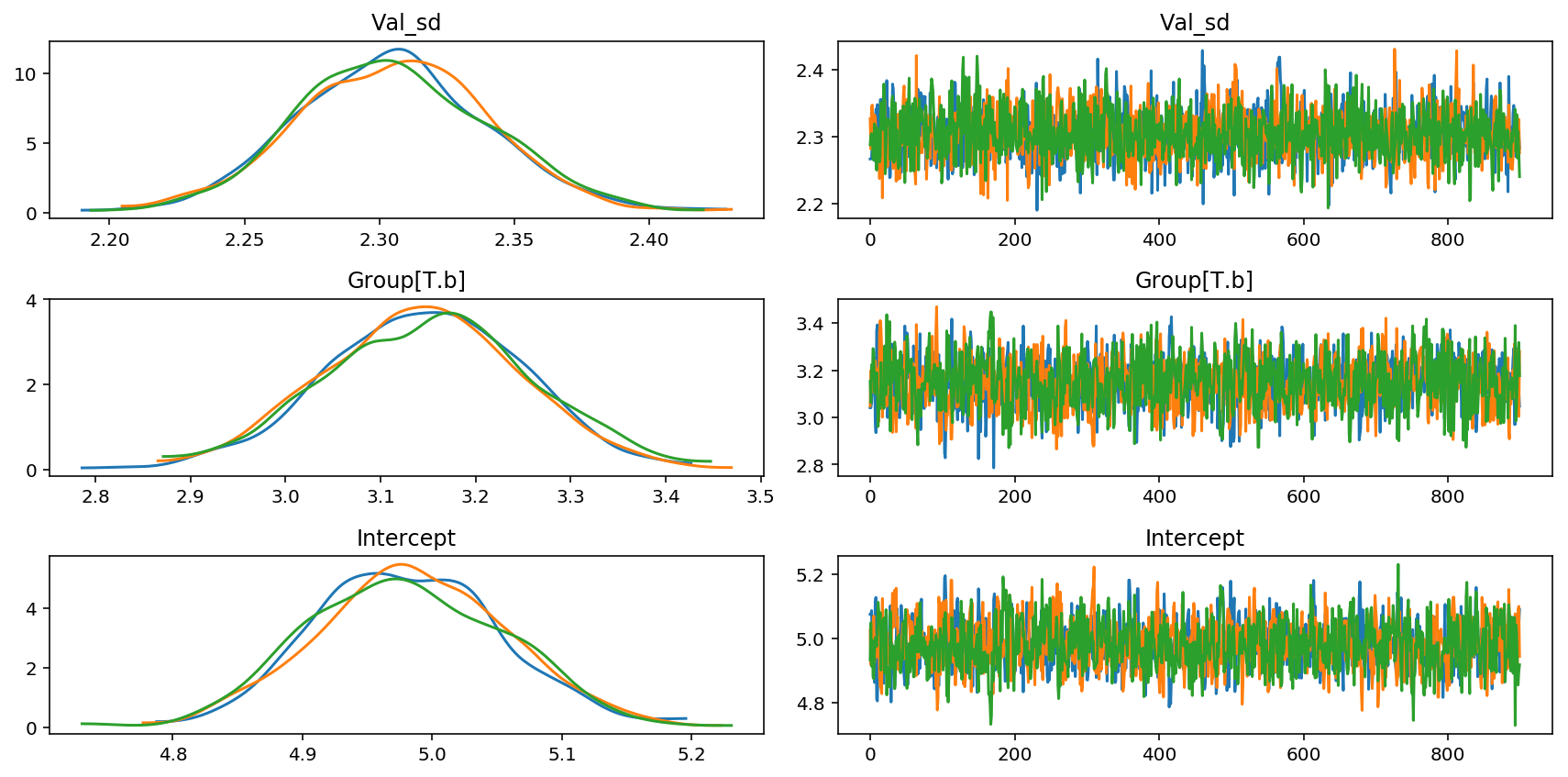
#Posterior plots removing first 100 samples for burn-in
res_b[100:].plot();
[96]:
res_b[100:].summary()
[96]:
| mean | sd | hpd0.95_lower | hpd0.95_upper | effective_n | gelman_rubin | |
|---|---|---|---|---|---|---|
| Group[T.b] | 3.145886 | 0.104301 | 2.936774 | 3.344979 | 1493 | 1.000435 |
| Intercept | 4.981076 | 0.072968 | 4.850235 | 5.129755 | 1415 | 1.000364 |
| Val_sd | 2.304672 | 0.035844 | 2.235005 | 2.376468 | 1881 | 0.999520 |
[97]:
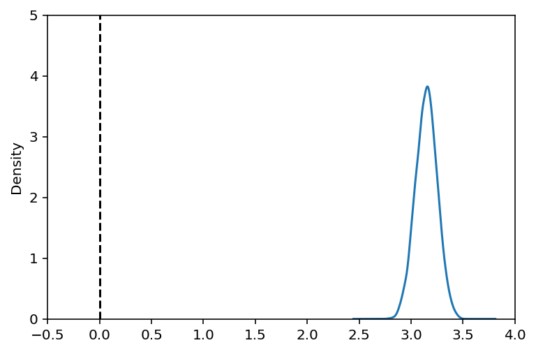
#Grab just the posterior of the term of interest (group)
group_posterior = res_b.to_df()['Group[T.b]']
ax = group_posterior.plot(kind='kde',xlim=[-.5,4],ylim=[0,5])
ax.axvline(0,0,3,linestyle='--',color='k');
[98]:
#Probabiliy that posterior is > 0
(group_posterior > 0).mean()
[98]:
1.0
Generate multi-level regression data
Generate data for a multivariate regression model with random intercepts and slope effect for each group
[51]:
# Simulate some multi-level data with pymer4
from pymer4.simulate import simulate_lmm
df, blups, coefs = simulate_lmm(num_obs=500, num_coef=2, num_grps=25, coef_vals=[5,3,-1])
df.head()
blups.head()
[51]:
| DV | IV1 | IV2 | Group | |
|---|---|---|---|---|
| 0 | 6.304926 | -0.610891 | -1.567181 | 1.0 |
| 1 | 9.350987 | 1.118879 | -0.072492 | 1.0 |
| 2 | 3.917564 | -0.919558 | -1.009021 | 1.0 |
| 3 | 2.390540 | -1.832521 | -0.850452 | 1.0 |
| 4 | -0.622128 | -1.382818 | 0.737954 | 1.0 |
[51]:
| Intercept | IV1 | IV2 | |
|---|---|---|---|
| Grp1 | 5.181938 | 2.930271 | -0.937849 |
| Grp2 | 5.176513 | 2.789747 | -1.283368 |
| Grp3 | 5.155200 | 3.143078 | -0.891992 |
| Grp4 | 5.215888 | 3.263981 | -1.136450 |
| Grp5 | 4.754923 | 2.589841 | -0.879531 |
Frequentist multi-level model
[52]:
# Fit multi-level model using pymer4 (lmer in R)
from pymer4.models import Lmer
model = Lmer('DV ~ IV1 + IV2 + (IV1 + IV2|Group)',data=df)
model.fit()
Formula: DV ~ IV1 + IV2 + (IV1 + IV2|Group)

Family: gaussian         Inference: parametric

Number of observations: 12500    Groups: {'Group': 25.0}

Log-likelihood: -17812.104       AIC: 35624.208

Random effects:

                 Name    Var    Std
Group     (Intercept)  0.079  0.281
Group             IV1  0.094  0.307
Group             IV2  0.070  0.265
Residual               0.989  0.995

               IV1  IV2   Corr
Group  (Intercept)  IV1  0.152
Group  (Intercept)  IV2 -0.081
Group          IV1  IV2 -0.329

Fixed effects:
[52]:
| Estimate | 2.5_ci | 97.5_ci | SE | DF | T-stat | P-val | Sig | |
|---|---|---|---|---|---|---|---|---|
| (Intercept) | 5.099 | 4.987 | 5.210 | 0.057 | 24.001 | 89.480 | 0.0 | *** |
| IV1 | 3.049 | 2.927 | 3.170 | 0.062 | 23.962 | 49.169 | 0.0 | *** |
| IV2 | -0.988 | -1.093 | -0.883 | 0.054 | 24.006 | -18.386 | 0.0 | *** |
[56]:
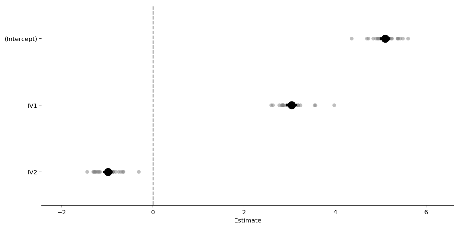
# Plot coefficients and the group BLUPs as well
model.plot_summary();
[81]:
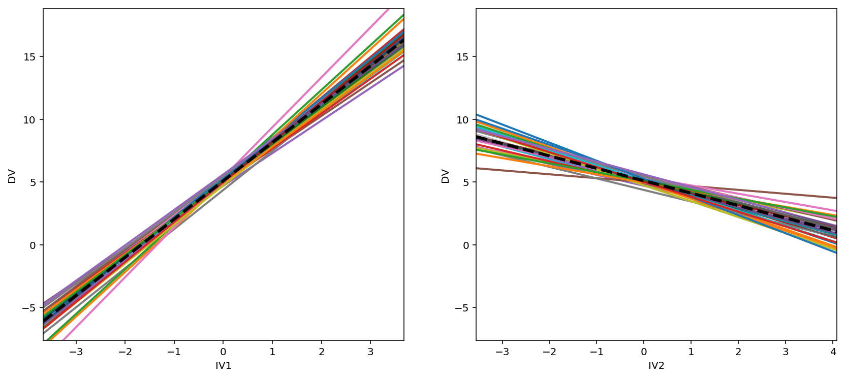
# Alternatively visualize coefficients as regression lines with BLUPs overlaid
f,axs = plt.subplots(1,2,figsize=(14,6));
model.plot('IV1',ax=axs[0],);
model.plot('IV2',ax=axs[1]);
Bayesian multi-level model
[57]:
b_model = Model(df)
results = b_model.fit('DV ~ IV1 + IV2',random=['IV1+IV2|Group'],samples=1000,chains=3)
Auto-assigning NUTS sampler...
Initializing NUTS using advi...
Average Loss = 17,878:  57%|█████▋    | 28265/50000 [00:41<00:32, 675.56it/s]
Convergence archived at 28300
Interrupted at 28,299 [56%]: Average Loss = 22,176
Multiprocess sampling (3 chains in 3 jobs)
NUTS: [DV_sd_interval__, IV2|Group_offset, IV2|Group_sd_log__, IV1|Group_offset, IV1|Group_sd_log__, 1|Group_offset, 1|Group_sd_log__, IV2, IV1, Intercept]
100%|██████████| 1500/1500 [02:04<00:00, 12.04it/s]
The number of effective samples is smaller than 25% for some parameters.
[59]:
b_model.backend.model
[59]:
[60]:
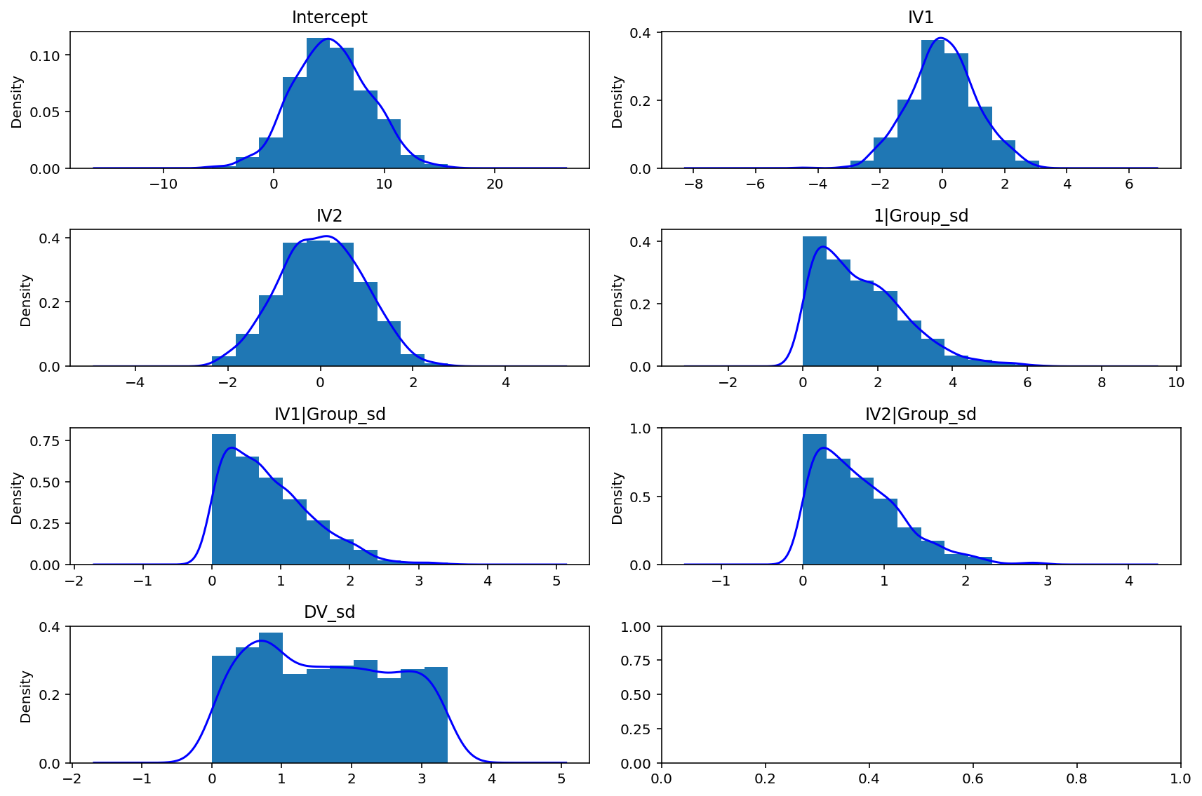
# Plot priors
b_model.plot();
/Users/Esh/anaconda3/lib/python3.6/site-packages/matplotlib/axes/_axes.py:6462: UserWarning: The 'normed' kwarg is deprecated, and has been replaced by the 'density' kwarg.
  warnings.warn("The 'normed' kwarg is deprecated, and has been "
/Users/Esh/anaconda3/lib/python3.6/site-packages/matplotlib/axes/_axes.py:6462: UserWarning: The 'normed' kwarg is deprecated, and has been replaced by the 'density' kwarg.
  warnings.warn("The 'normed' kwarg is deprecated, and has been "
/Users/Esh/anaconda3/lib/python3.6/site-packages/matplotlib/axes/_axes.py:6462: UserWarning: The 'normed' kwarg is deprecated, and has been replaced by the 'density' kwarg.
  warnings.warn("The 'normed' kwarg is deprecated, and has been "
/Users/Esh/anaconda3/lib/python3.6/site-packages/matplotlib/axes/_axes.py:6462: UserWarning: The 'normed' kwarg is deprecated, and has been replaced by the 'density' kwarg.
  warnings.warn("The 'normed' kwarg is deprecated, and has been "
/Users/Esh/anaconda3/lib/python3.6/site-packages/matplotlib/axes/_axes.py:6462: UserWarning: The 'normed' kwarg is deprecated, and has been replaced by the 'density' kwarg.
  warnings.warn("The 'normed' kwarg is deprecated, and has been "
/Users/Esh/anaconda3/lib/python3.6/site-packages/matplotlib/axes/_axes.py:6462: UserWarning: The 'normed' kwarg is deprecated, and has been replaced by the 'density' kwarg.
  warnings.warn("The 'normed' kwarg is deprecated, and has been "
/Users/Esh/anaconda3/lib/python3.6/site-packages/matplotlib/axes/_axes.py:6462: UserWarning: The 'normed' kwarg is deprecated, and has been replaced by the 'density' kwarg.
  warnings.warn("The 'normed' kwarg is deprecated, and has been "
[61]:
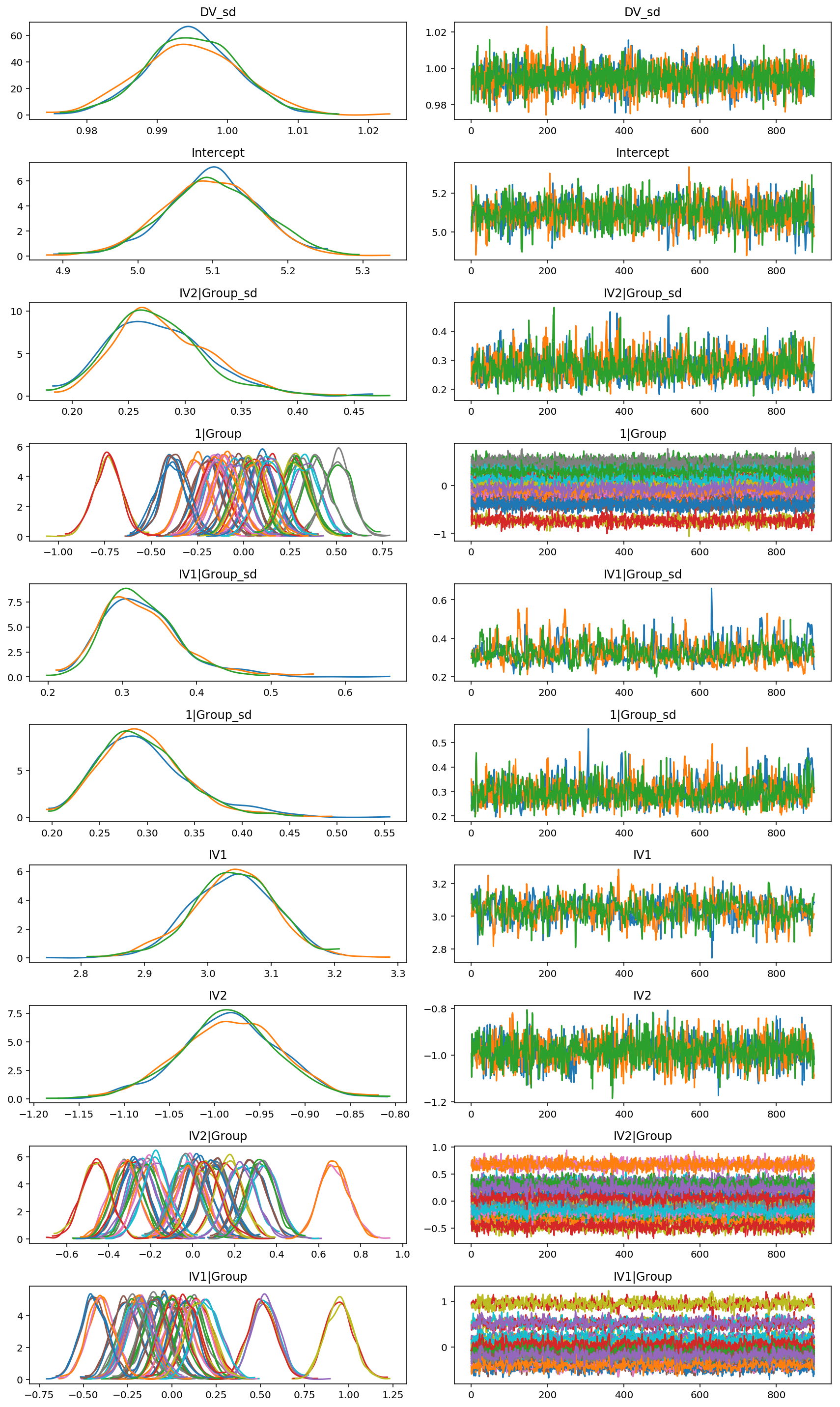
#Plot posteriors
results[100:].plot();
[63]:
results[100:].summary()
[63]:
| mean | sd | hpd0.95_lower | hpd0.95_upper | effective_n | gelman_rubin | |
|---|---|---|---|---|---|---|
| 1|Group_sd | 0.296123 | 0.046973 | 0.213154 | 0.394314 | 569 | 1.000344 |
| DV_sd | 0.994745 | 0.006591 | 0.981409 | 1.007187 | 2700 | 0.999791 |
| IV1 | 3.039772 | 0.065466 | 2.905801 | 3.164539 | 592 | 0.999766 |
| IV1|Group_sd | 0.325975 | 0.052205 | 0.236429 | 0.434760 | 500 | 0.999868 |
| IV2 | -0.983000 | 0.054667 | -1.102063 | -0.885895 | 1421 | 0.999686 |
| IV2|Group_sd | 0.277549 | 0.043083 | 0.200689 | 0.365828 | 977 | 1.002444 |
| Intercept | 5.098220 | 0.062943 | 4.972299 | 5.217102 | 1570 | 1.000099 |
[76]:
#Plot all posterior on the same plot
results_df = results.to_df()
fixed_terms = [col for col in results_df.columns if '|' not in col and 'sd' not in col]
results_df = results_df[fixed_terms]
results_df.plot(kind='kde',xlim=[-2,6],figsize=(8,6)).axvline(0,color='k',linestyle='--')
[76]:
<matplotlib.lines.Line2D at 0x125d59400>
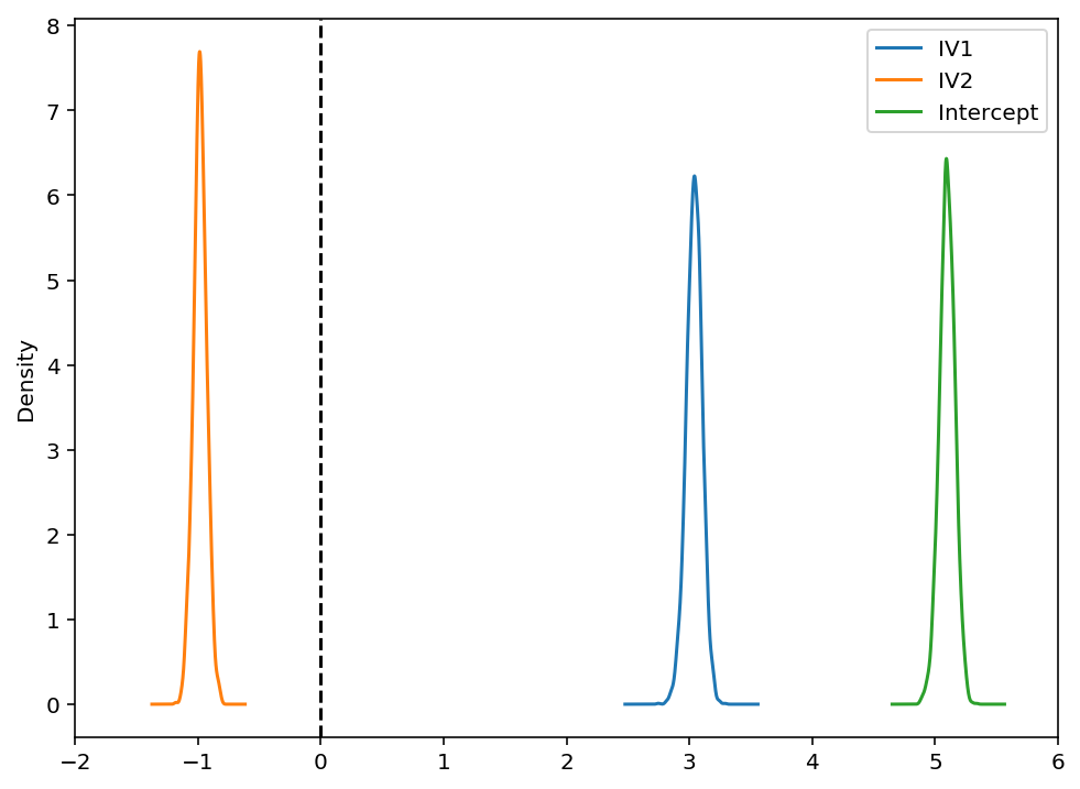
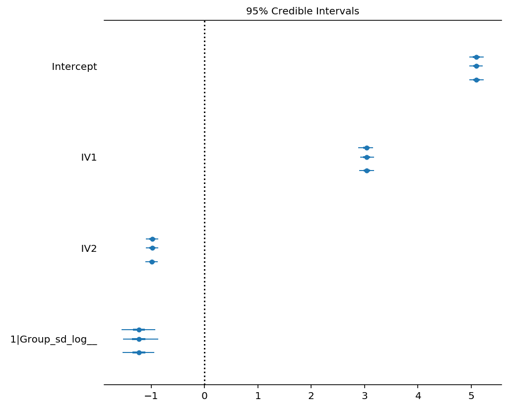
Because we used pymc3 for the backend estimation in bambi, we have access to few extra goodies. Here we make a forest plot similar to the one above for the frequentist model, but with 95% credible intervals instead
[73]:
# Credible interval plot using pymc3
# Line line is 95% credible interval calculated as higher posterior density
# Inter quartile range is thicker line
# Dot is median
f,ax = plt.subplots(1,1,figsize=(8,6))
pm.forestplot(b_model.backend.trace,varnames=list(map(str,b_model.backend.model.vars[:4])),rhat=False)
[73]:
<matplotlib.gridspec.GridSpec at 0x11a911ba8>
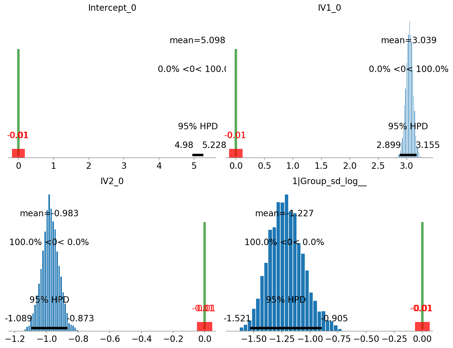
We can also plot the posterior overlayed with a region of practical equivalence (ROPE), i.e. range of values that were the coefficients to fall into, we might interpret them differently. We can see that all our posterior distributions fall outside of this range.
[75]:
# Show credible interval cutoffs, and also overlay region of practical equivalence (arbitrary, in this case close enough to 0 to not matter)
pm.plot_posterior(b_model.backend.trace,
                  varnames=list(map(str,b_model.backend.model.vars[:4])),
                  ref_val=0,
                  text_size = 14,
                  rope=[-.01,.01],
                  figsize=(10,8));
